en-USel-GRes-ES
Menu

Appendix C


Materials
To be continued >
Introduction

Subject description

Simple one-storey structure comprising four columns whose tops are connected by a rigid slab-diaphragm

In general, when a horizontal force H acts on a storey level, all the points of the slab including the column tops move in accordance with the same rules due to the in-plane rigidity of the slab.

These rules induce the diaphragm to develop a parallel (translational) displacement by δxo, δyo and a rotation θabout the a point CT(xCT, yCT, the centre of stiffness, in the xCy coordinate system, which has as origin the point Cand is rotated with respect to the initial coordinate system X0Y by an angle a.


Coordinate systems

Χ0Υ     initial coordinate system
x’0y’     auxiliary coordinate system
xCTy    principal coordinate system

Parallel translation in both directions
and rotation of the diaphragm, due to force H

Axis transformation


ζ= x·cosφ+y·sinφ

η=-x·sinφ+y·cosφ


x=ζ·cosφ-η·sinφ

y=ζ·sinφ+η·cosφ


x-vector:

ζ=x·cosφ & η=-x·sinφ


y-vector:

ζ=y·sinφ & η=y·cosφ


Relationships of axis transformation due to rotation

Case 1: Translation of centre of stiffness CT along x direction by δxο

When a horizontal force Hx acts on the CT along the x direction, the 3 following equilibrium equations should apply:

·         The sum of forces acting in x direction is be equal to Hx, i.e. Hx=Σ(Vxxoi)                        (i)

·         The sum of forces acting in y direction is equal to zero, i.e. Σ(Vxyoi)=0.0                         (ii)

·         The sum of moments Vxxoi and Vxyoi  about point CT is equal to zero,      
           i.e. Σ(Vxxoi·yi-Vxyoi·xi)=0                                                                                                      (iii)

where Vxyoi=δxo·Kxyi with Kxyi=1/2·(Kζi-Kηi)·sin2φi   and φi=φi-a

 Expression (i) yields Hx=Σ(δxo·Kxxi)=δxo·Σ(Kxxi)  where  

Because of the identity sin (w1-w2)=sinw1·cosw2-cosw1·sinw2, Kxyi=1/2·(Kζi-Kηi)·(sin2φi·cos2a-cos2φi·sin2a) equation (ii) becomes Σ(Kxyi)=0 Σ[(Kζi-Kηi)·sin2φi·cos2a]=Σ[(Kζi-Kηi)cos2φi·sin2a] cos2a·Σ[(Kζi-Kηi)·sin2φi]=sin2a·Σ[(Kζi-Kηi)·cos2φi]

                                                                (3)

The angle a of the principal system is calculated from this expression. However, the coordinates xCT, yCT of CT are still unknown. It is possible, though, to work on the auxiliary system x’0y’ which is parallel to the xCTy and has the advantage that its stiffnesses are the same with the ones of the final principal system xCTy. Therefore, coordinates X,Y are transferred to the x’,y’.

Example:

Calculation of angle a of the principal system :

Using the same values for Kζ, Kη previously calculated and since 2φ1=2φ2=0˚, 2φ3=60˚ and 2φ4=90˚:

(3) tan2a=Σ[(Kζi-Kηi)·sin2φi]/Σ[(Kζi-Kηi)·cos2φi]

tan2a=[(31.1-31.1)·106·sin0˚ +(31.1-31.1)·106·sin0˚+(186.6-26.2)·106·sin60˚+ (19.7-78.7)·106·sin90˚]/

/[( 31.1-31.1)·106·cos0˚+(31.1-31.1)·106·cos0˚ + (186.6-26.2) ·106·cos60˚+ (19.7-78.7)·106·cos90˚]= =[0+0+138.9-59.0]/[0+0+80.2+0.0]=79.9/80.2=0.996 2a=44.88˚ a=22.44˚

Therefore the angle of the principal system is a=22.44˚

Coordinate system transformation: From the initial system X0Y we are transferred to the auxiliary x’0y’, which is parallel to the principal system xCTy, therefore angle of the initial system is a=22.4˚:

 sina=0.3817, cosa=0.9243

C1: from C1(0,0) and φ1=0˚ becomes C1(0,0) φ1=-22.44˚

C2: from C2(6.0,0) and φ2=0˚ becomes C2(6.0·0.924=5.544, -6.0·0.3817=-2.290), φ2=-22.44˚

C3: from C3(0.0,5.0) and φ3=30˚  becomes C3(5.0·0.3817=1.9085, 5.0·0.924=4.62), φ3=30˚-22.44˚ =7.56˚ C3(5.544, -2.290), φ3=7.56˚

C4: from C4(6.0, 5.0) and φ4=45˚  becomes C4(6.0·0.924+5.0·0.3817=7,4542, -6.0·0.3817+5.0·0.9243=2.331), φ4=45˚-22.44˚ =22.56˚ C4(7.454, -2.331), φ4=22.56˚

CM: from CM(3.0, 2.5) becomes CM(3.0·0.924+2.5·0.3817=3.727, -3.0·0.3817+2.5·0.9243=1.166)


Working on the auxiliary coordinate system x’0y’

xi=x’i-x’CT and yi=y’i-y’CT  therefore equation (iii) yields:

δxo·Σ((y’i-yo)·Kxxi-(x’i- x’CT)·Kxyi)=0 Σ(y’i·Kxxi)-yo·Σ(Kxxi)-Σ(x’i·Kxyi)+ x’CT·Σ(Kxyi)=0

Σ((x’i- x’CT)·Kyyi-(y’i- y’CT)·Kxyi)=0 -Σ(y’i·Kxyi)+ y’CT ·Σ(Kxyi)+Σ(x’i·Kyyi)- x’CT·Σ(Kyyi)=0.

Since Σ(Kxyi)=0, Σ(y’i·Kxxi)- y’CT·Σ(Kxxi)-Σ(x’i·Kxyi)=0 → 

-Σ(y’i·Kxyi)+Σ(x’i·Kyyi)- x’CT·Σ(Kyyi)=0 → 


Case 2: Translation of centre of stiffness CT along direction y by δyο

Accordingly, taking into account that Kyxi=Kxyi, the corresponding expressions are:

 where ,       

Therefore the final relationships are:

,   where                             (4)

,   where                            (5)

Example:

Columns stiffnesses in the principal system xCTy:

Since C1, C2 have a square cross section Kxx1=Kyy1=Kxx2=Kyy2=31.1·106 N/m, Kxy1=Kxy2=0.0

C3: φ3=7.56˚ (a) Kxx3= Kζ3·cos2φ3+Kη3·sin2φ3 =[186.6·0.99132+26.2·0.13162]·106=183.82·106 N/m

(b)   Kxy3=(1/2)·(Kζ3-Kη3)·sin2φ3=0.5·(186.6-26.2)· 106·0.261=20.93·106 N/m

(d) Kyy3= Kζ3·sin2φi+Kη3·cos2φ3 =[186.6·0.13162+26.2·0.99132] ·106 N/m =28.98·106 N/m

C4: φ4=22.56˚ (a) Kxx4=Kζ4·cos2φ4+Kη4·sin2φ4=[19.7·0.92352+78.7·0,38372] ·106=28.39·106 N/m

(b)   Kxy4=(1/2)·(Kζ4-Kη4)·sin2φ4=0.5·(19.7-78.7)·106·0.709=-20.92·106 N/m

(d) Kyy4= Kζ4·sin2φi+Kη4·cos2φ3 =[19.7·0,38372+78.7·0.92352] ·106=70.02·106 N/m

Total stiffnesses of the diaphragm and structural moments of the stiffnesses with respect to  CT :

Kxx=Σ(Kxxi)=( 31.1+31.1+183.82+28.39) ·106=274.41·106 N/m

Kyy=Σ(Kyyi)= (31.1+31.1+28.98+70.02) ·106=161.2·106 N/m

Σ(x’i·Kyyi)=[0.0·31.1+5.544·31.1+1.9085·28.98+7.4542·70.02]·106 =749.55·106 N

Σ(x’i·Kxyi)=[0.0·0+5.544·0+1.9085·20.93+7.4542·(-20.93)]·106=-116.07·106 N

Σ(y’i·Kxxi)=[0.0·31.1 -2.29·31.1 +4.62·183.82+2.331·28.39]·106=844.21·106 N

Σ(y’i·Kxyi)= [0.0·0.0 -2.29·0.0 +4.62·20.93+2.331· (-20.92)]·106=47.93·106 N

x’CK=[Σ(x’i·Kyyi)-Σ(y’i·Kxyi)]/Σ(Kyyi)=( 749.55-47.93)/161.2=4.353 m

y’CK=[Σ(y’i·Kxxi)-Σ(x’i·Kxyi)]/Σ(Kxxi)=( 844.21+116.07)/274.41=3.500 m


Case 3: Rotation of the diaphragm by an angle θz about CT

Displacements due to rotation from a moment M
applied in CT

Displacements of a random point i of the diaphragm due to rotation by θz

δi=ri·θz

δxi =-δi·sinωi

sinωi =yi /ri

δxi =-ri·θz·yi/ri=-yi·θz

δyi=xi·θz

Consider the principal coordinate system xCTy

The deformation induced by the external moment M applied in CT , is examined. In order to examine this deformation a transfer is needed from the auxiliary system x’0y’ to the principal system xCTy by a simple parallel translation.  By also transferring the centre of mass in the principal system as well, the structural eccentricities eox, eoy of CM with respect to CT, derive from the expressions:

 ,  , ,                                        (6)

The deformation of the diaphragm is a rotation θz about CT. Rotation θz of diaphragm induces a displacement δi at the top of each column i with coordinates xi,yi with respect to the coordinate system having as origin CT. If the distance of point i from CT is ri, the two components of the (infinitesimal) deformation δi are: δxi=-θz·yi and δyi= θz·xi

Example:

Coordinate transfer in the principal system and calculation of the structural eccentricities :

Expressions (6) yield:

C1(0.0-4.353=-4.35, 0.0-3.500=-3.50) φ1=-22.44˚                Kxx=31.1·106, Kyy=31.1·106, Kxy=0.0

C2(5.544-4.353=1.19, -2.290-3.500=-5.79), φ2=-22.44˚                   Kxx=31.1·106, Kyy=31.1·106, Kxy=0.0

C3(1.9085-4.353=-2.44, 4.62-3.500=1.12), φ3=7.56˚                        Kxx=183.82, Kyy=28.98, Kxy=20.93

C4(7,4542-4.353=3.10, 2.3312-3.500=-1.17), φ4=22.56˚      Kxx=28.39, Kyy=70.02, Kxy=-20.92

CM(3.727-4.353=-0.626, 1.166-3.500=-2.334) and obviously CT(0,0)

eox=-0.626 m, eoy=-2.334 m


Displacements δxi, δyi incuce shear forces Vxi and Vyi in each column:

Vxi=Kxxi·δxi= Kxxi·(-θz·yi ) Vxi= -θz·Kxxi·yi and            Vyi=Kyyi·δyi=kyyi·θz·xi             Vyi=θz·kyyi·xi

The resultant of the moments of all shear forces Vxi, Vyi with respect to the CT should be equal to the external moment MCT i.e.:

MCT=Σ[-Vxi·yi + Vyi·xi+Kzi] MCT= θz·Σ[Kxxi·yi2 + Kyyi·xi2+Kzi]  

  where                                                        (7)

Example:

Calculation of diaphragm torsional stiffness:

Κθ=Σ(Kxxi·yi2+Kyyi·xi2+Kzi)=Σ[31.1·3.52+31.1·4.352+31.1·5.792+31.1·1.192+183.82·1.122+ 28.98·2.442+28.39·1.172+70.02·3.102]·106 N·m= =[381.0+588.5+1042.6+44.0+230.6+172.5+38.9+672.9] ·106 N·m Κθ=3174·106 N·m

The quantity Κθ=Σ(Kxxi·yi2 + Kyyi·xi2+Kzi) is called torsional stiffness of the diaphragm, measured in units of moment e.g. N·m, by analogy with the quantities Kx=Σ(Kxi), Ky=Σ(Kyi) which are called lateral stiffnesses of the diaphragm in direction x and y respectively and measured in N/m. The torsional stiffness of the column itself is usually insignificant and can be ignored (§5.4.3.4).

Definitions:

Lateral stiffness Κjk of diaphragm denotes the force in j direction required to cause displacement of the diaphragm by one unit in the k direction.

Torsional stiffness Κθ of diaphragm denotes the moment required to cause rotation of the diaphragm by one unit.

Torsional stiffness ellipse, torsional radii


Question: Create a simple idealised equivalent structural system with the same seismic behaviour as the actual structural system.

Solution: Four idealised columns E1, E2 and E3, E4 are placed symmetrically with respect to the centre CT and to the axes x and y, i.e. all four idealised columns have x and y coordinates with the same absolute values. Each idealised column is assumed to have a stiffness equal to Kx=1/4·Σ(Kxi) and Ky=1/4·Σ(Kyi).

This system satisfies the two conditions of the actual system, concerning the translations of all diaphragm columns since:

Stiffness by x: 4·1/4·Σ(Kxi)=Σ(Kxi) and stiffness by y: 4·(1/4)·Σ(Kyi)=Σ(Kyi).

To satisfy the third condition, the torsional stiffness of the idealised system should be

Kθ,eq=[Kx1·y2+Kx2·y2+Ky1·x2+Ky2·x2]=Σ(Kxxi)·y2+Σ(Kyyi) ·x2

equal to the torsional stiffness of the actual system

Kθ,re=Kθ=Σ(Kxxi·yi2 + Kyyi·xi2-2Kxyi·xi·yi+Kzi),

i.e. should Kθ,eq= Kθ,re à Σ(Kxxi)·y2+Σ(Kyyi)·x2=Kθ à

                            where  and                          (8)

The curve equation (8) is an ellipse with centre CT and semiaxes rx, ry oriented along the principal axes

Example C.6:

Calculation of the torsional stiffness ellipse

rx=√(Kθ/Kyy)=√(3134·106N·m /161.2·106N/m)=4.41 m

ry=√(Kθ/Kxx)=√(3134·106 N·m /274.41·106N/m)=3.38 m

Conclusion:

The torsional behaviour of a floor can be described by the torsional stiffness ellipse (CT, rx, ry) which represents the equivalent distribution of the diaphragm stiffness.

The radii rx, ry, of the ellipse are called torsional radii.

There are infinite solutions of idealised dual system sets, whose most characteristic is the one with the four idealised columns placed in the four ellipse ends.

Generally, there are infinite solutions with n-tuple diametrically opposed systems, where each idealised column stiffness is equal to 1/n of the total system stiffness.


Superposition of the three cases

So far, all the calculations depended on the structure geometry and were not affected by the magnitude of the external loading. For instance the centre of stiffness, the structural eccentricities, and the torsional radii, are independent of the seismic force magnitude.

Next, the displacements and stress resultants of the structure, due to external seismic loading H, will be calculated.

The relevant seismic force H is applied at the centre of mass CM of the diaphragm. This force is resolved in two forces Hx and Hy parallel to the two axes of the principal system. In order to apply the previous analysis, the forces Hx, Hy are transferred to the centre of stiffness CT together with the moment MCT according to the expression:

                                                                                                        (9)

Example C.7-1: Given a horizontal force in x direction equal to is H=90.6 kN, carry-out the analysis of the structure.

Calculation of moment MCT :

The structural eccentricities are eox =-0.626 and eoy= yCM=-2.334m

For a given force Η=HX=90.6 kN in the initial system X0Y, the equivalent loading in the principal system (a=22.44ο) is: Hx=HX·cosa=90.6·0.924=83.72 kN and Hy=-HX·sina=-90.6·0.382=-34.64 kN and

ΜCT=-Hx·eoy+Hy·eox=-83.72kN·(-2.334m)+[-34.64kN·(-0.626m)]=195.4 kNm+21.7kNm=217.1 kNm


The following quantities are calculated using the Hx, Hy, MCT:

·         the displacements  δxo, δyo and θz of CT using the expressions:

              ,  ,                                                                          (10)

where  , ,  

Example C.7-2:

Quantities Kxx=Σ(Kxxi)= 161.2·106N/m, Kyy=Σ(Kyyi)= 161.2·106 N/m and Κθ=3134·106 N·m are already calculated therefore:

δxo=Hx/Κxx =83.72·103N/(274.41·106N/m)=0.305 mm,

δyo=Hy/Κyy =-34.46·103N/(161.2·106 N/m)=- 0.214 mm and

θz=MCT/Kθ=217.1kNm/(3134·103kNm)=0.692·10-4 

·         the displacements δxi, δyi of the top of each column using the expressions:

,                                                 (11)

·         and the displacements δζi, δηi by transferring δxi, δyi to the local system of each column using the expressions:

,   where                        (12)

Example C.7-3:

C1: δx1= δxo- θz·y1=0.305mm-0.692·10-4·(-3.50·103mm)=(0.305+0.242)mm=0.547 mm

δy1= δyo+ θz·x1=-0.214mm+0.692·10-4·(-4.35·103mm)=(-0.214-0.301)mm=-0.515 mm

By transferring to the local system where φ1=0.0-22.44°=-22.44°.

δζ1= δx1·cosφ1+δy1·sinφ1=0.547·0.924-0.515·(-0.382)=0.505+0.197=0.702 mm

δη1=-δx1·sinφ1+δy1·cosφ1=-0.547·(-0.382)+(-0.515)·0.924=0.209-0.476=-0.267 mm

C2: δx2= δxo- θz·y2=0.305mm-0.692·10-4·(-5.79·103mm)=(0.305+0.400)mm=0.705 mm

δy2= δyo+ θz·x2=-0.214mm+0.692·10-4·1.19·103mm=(-0.214+0.082)mm=-0.132  mm

By transferring to the local system where φ2=0.0-22.44°=-22.4°.

δζ2= δx2·cosφ2+δy2·sinφ2=0.705·0.924+(-0.291)·(-0.132)=0.652+0.038=0.701 mm

δη2=-δx2·sinφ2+δy2·cosφ2=-0.705·(-0.382)+(-0.132)·0.924=0.269-0.122=0.147 mm

C3: δx3= δxo- θz·y3=0.305mm-0.692·10-4·1.12·103mm=(0.305-0.078)mm=0.227 mm

δy3= δyo+ θz·x3=-0.214mm+0.692·10-4·(-2.44·103mm)=(-0.214-0.169)mm=-0.383 mm

By transferring to the local system where φ3=30.0-22.44°=7.56°.

δζ3= δx3·cosφ3+δy3·sinφ3=0.227·0.991+(-0.383)·0.132=0.225-0.050=0.175 mm

δη3=-δx3·sinφ3+δy3·cosφ3=-0.227·0.132+(-0.383)·0.991=-0.030-0.380=-0.410 mm

C4: δx4= δxo- θz·y4=0.305mm-0.692·10-4·(-1.17·103mm)=(0.305+0.081)mm=0.386 mm

δy4= δyo+ θz·x4=-0.214mm+0.692·10-4·3.10·103mm=(-0.214+0.215)mm=0.001 mm

By transferring to the local system where φ4=45.0-22.44°=22.56°.

δζ4= δx4·cosφ4+δy4·sinφ4=0.386·0.923+0.001·0.384=0.355+0.000=0.355 mm

δη4=-δx4·sinφ4+δy4·cosφ4=-0.386·0.384+0.001·0.923=-0.148+0.001=-0.147 mm

In the example considered, for seismic action in X direction, the deformation due to rotation at column C2 gives δx2,θ=0.400 mm, higher than the deformation  due to translation δxo=0.305 mm. The total displacement is therefore δx2=0.305+0.400=0.705 mm.

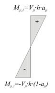
     Figure C.7: Moment distribution (Mji,1- Mji,2=Vji·h)

·        shear forces and bending moments of each column in its local system based on the relationships

                                                 ,                                                   (13)

                ,                              (14)

            ,  


Example C.7-4:

Calculation of shear forces and bending moments :

The moment distribution factor is assumed the same in both directions aζi=aηi=0.50

C1: Vζ1=δζ1·Kζ1=0.702mm·31.1·106 N/m =21.8 kN

Vη1=δη1·Kη1=-0.267mm·31.1·106 N/m =-8.3 kN

Mζ1,1 =Vζ1·h·0.50=21.8·3.0·0.50=32.7 kNm              Mζ1,2=- Mζ1,1=-32.7 kNm

Mη1,1=Vη1·h·0.50=-8.3·3.0·0.50=-12.5 kNm              Mηι,2=- Mη1,1=12.5 kNm

C2: Vζ2=δζ2·Kζ2=0.701mm·31.1·106 N/m =21.8 kN

Vη2=δη2·Kη2=0.147mm·31.1·106 N/m =4.6 kN

Mζ2,1=Vζ2·h·0.50=21.8·3.0·0.50=32.7 kNm               Mζ2,2=- Mζ2,1=-32.7 kNm

Mη2,1=Vη2·h·0.50=4.6·3.0·0.50=6.9 kNm                  Mη2,2=- Mη2,1=-6.9 kNm

C3: Vζ3=δζ3·Kζ3=0.175mm·186.6·106 N/m =32.7 kN

Vη3=δη3·Kη3=-0.410mm·26.2·106 N/m =-10.8 kN

Mζ3,1=Vζ3·h·0.50=32.7·3.0·0.50=49.1 kNm               Mζ3,2=- Mζ3,1=-49.1 kNm

Mη3,1=Vη3·h·0.50=-10.8·3.0·0.50=-16.2 kNm                        Mη3,2=- Mη3,1=16.2 kNm

C4: Vζ4=δζ4·Kζ4=0.355mm·19.7·106 N/m =7.0 kN

Vη4=δη4·Kη2=-0.147mm·78.7·106 N/m =-11.6 kN

Mζ4=Vζ4·h·0.50=7.0·3.0·0.50=10.5 kNm                   Mζ4,2=- Mζ4,1=-10.5 kNm

Mη4,1=Vη4·h·0.50=-11.6·0·0.50=-17.4 kNm               Mη4,2=- Mη4,1=17.4 kNm

One-storey space frame with rectangular columns in random arrangement

Frame and model of a single-storey space frame

The analysis of the one-storey space frame illustrated in the figure, under horizontal seismic force H=90.6 kN is performed by means of four methods: (i) analysis using manual calculations, assuming fixed-ended columns, (ii) analysis using the Excel file, assuming fixed-ended columns, (iii) analysis using the Excel file, assuming columns with k=6, (iv) assuming using software, assuming actual beam and column torsional stiffnesses.

Analysis

(i)            Analysis using manual calculations, assuming fixed columns (k=12)

This method was described via the example presented to all previous paragraphs of this appendix.

(ii)          Analysis using the Excel file, assuming fixed-ended columns (k=12)

The related <diaphragm_general.xls> spreadsheet is used assuming fixed-ended columns.

The results are identical to those of the practical calculations.

The torsional stiffness ellipse and the equivalent columns of the structure are drafted at the end of the spreadsheet.

(iii)         Analysis using the Excel file, assuming columns with k=6

The centre of stiffness, the torsional radii and the stress resultants derived from this method are exactly the same as those of the previous methods, with the exception of deformations, whose their relative values, however, remain constant 12/6=2.00.

(iv)         Analysis using software, assuming actual beam and column torsional stiffnesses

In order to define the diaphragmatic function of a building’s storey, with actual stiffness and not with assumption of fixed function of its columns, it is necessary to use the appropriate software. Structural analysis software is necessary for one storey, as well as multistorey buildings, even in case of rectangular columns in parallel arrangement.

The method which describes the diaphragmatic behaviour of each floor is presented in Appendix D and this example is analysed as example 1.